Shannon Information Entropy for Seismic Reliability Assessment of Structures Using Self-Organizing Neural Networks
© 2020 Mostafa AllamehZade, et al. This is an open-access article distributed under the terms of the Creative Commons Attribution License, which permits unrestricted use, distribution, and reproduction in any medium, provided the original author and source are credited.
Abstract
Localization and quantification of structural damages and find a failure probability is the key important in reliability assessment of structures. In this study, a Self-Organizing Neural Network (SONN) with Shannon Information Entropy simulation is used to reduce the computational effort required for reliability analysis and damage detection. To this end, one demonstrative structure is modeled and then several damage scenarios are defined. These scenarios are considered as training datasets for establishing a Self-Organizing Neural Network model. In this regard, the relation between structural responses (input) and structural stiffness (output) is established using Self-Organizing Neural Network models. The established SONN is more economical and achieves reasonable accuracy in detection of structural damages under ground motion. Furthermore, in order to assess the reliability of structure, five random variables are considered. Namely, columns’ area of first, second and third floor, elasticity modulus and gravity loads. The SONN is trained by Shannon Information Entropy simulation technique. Finally, the trained neural network specifies the failure probability of purposed structure. Although MCS can predict the failure probability for a given structure, the SONN model helps simulation techniques to receive an acceptable accuracy and reduce computational effort.
Introduction
The main reason of structural failure is a sudden damage. In the past decades, special attention was given to avoid the unexpected failure of structural components by damage detection in structures in the early states. To this end, in recent years, various developments of non-destructive techniques based on changes in the structural responses have been widely published. They can only detect the presence of damage but also identify the location and the quantification of the damage. Additionally, the need to be able to detect in the early stages the presence of damage in complex structures and infrastructure has led to the increase of non-destructive techniques and new developments. During the past decades, many researches has been studying to purpose different and efficient techniques. Friswell presented a brief overview of the use of inverse methods in damage detection and location from response data [1]. A review based on the detection of structural damage through changes in frequencies has been discussed by Salawu [2]. However, in the presentence of complicated structures, many of them are not applicable. Therefore, the methods that are much more economical to achieve reasonable accuracy are always required. In recent years, there has been a growing interest in using Artificial Neural Networks (ANNs), a computing technique that works in a way similar to that of biological nervous systems. Many researchers used ANN to study a beam using multilayer perceptron (MLP) ANN [3,4]. Furthermore, another application of ANN is to evaluation of the failure probability and safety levels of structural systems.Bakhshi and Vazirizade used a radial network in order to predict the stiffness of the each member in a frame according to its response to a record [5]. In fact, they showed ANN can provide a mapping from the maximum story drifts to columns stiffness. Gomes et al. and Bucher used ANN for obtaining the failure probability for a cantilever beam and compared ANN with other conventional methods [6,7]. They found that ANN methods that can approximate the limit state function may decrease the total computational effort on the reliability assessment, but more studies, including large systems with non-linear behavior must be studied. Elhewy et al. studied about the ability of ANN model to predict the failure probability of a composite plate [8]. They compared the performance of the ANN-based RSM (Response Surface Methods) (ANN-based FORM and ANN-based MCS) with that of the polynomial-based RSM. Their results showed that the ANN-based RSM was more efficient and accurate than the polynomial-based RSM. It was shown that the RSM may not be precise when the probability of failure was extremely small as well as the RSM requires a relatively long computation time as the number of random variables increases [9,10]. Zhang and Foschi employed ANN for seismic reliability assessment of a bridge bent with and without seismic isolation, but in that case they used explicit limit states [11]. However, most of them are utilized explicit and approximate limit states and more focused on the reliability assessment of components by ANN. In this regard, this study is focused on two separate parts; (1) localization and quantification of structural damages using ANN; (2) seismic reliability assessment of one steel structure using ANN-based Shannon Information Entropy simulation.
Self-Organizing Neural Network (SONN)
Pattern recognition is a branch of machine learning that focuses on the recognition of patterns and regularities in data, although it is in some cases considered to be nearly synonymous with machine learning. Pattern recognition systems are in many cases trained from labeled “training” data (supervised learning), but when no labeled data are available other algorithms can be used to discover previously unknown patterns (unsupervised learning).
Typically the categories are assumed to be known in advance, although there are techniques to learn the categories (clustering). Methods of pattern recognition are useful in many applications such as information retrieval, data mining, document image analysis and recognition, computational linguistics, forensics, biometrics and bioinformatics
In Pattern Recognition applications many algorithms and models have been proposed for seismology, especially for clustering, regression and classification between earthquakes and explosions. Applications in which a training data set with categories and attributes is available and the goal is to assign a new object to one of a finite number of discrete categories are known as supervised classification problems [12]. We present the use of the SONN and Shannon Information Entropy simulation as an alternative for modeling earthquakes aftershocks distribution. They are suitable tools in statistics for modeling multiple dependence such as earthquakes. For this reason, they have been widely used in earthquake prediction, and more recently in other fields such as geophysics, oceanography, hydrology, geodesy
Self-Organizing Feature Mapping (SOFM) algorithm is an unsupervised-learning process. The SOFM defines a mapping from the input data space on to an output layer by the processing units of e.g. 2-D laminar. Kohonen’s algorithm creates a vector quantizer by adjusting weights from common input nodes to M output nodes arranged in a two dimensional grid as shown in Figure. 3.
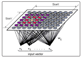
Figure 3: Two-dimensional array of output nodes used to form feature maps
Weights between input and output nodes are initially set to small random values and an input is presented.
For building the Kohonen layer, two steps should be considered. First, to make sure that the weight vectors of the neurodes in the layer are properly initialized. Second, the weight vectors and input vectors should be normalized before its use to a constant, fixed length usually one.
Only two-dimensional inputs with the weight vectors to unit length have been used. Each neurode in the Kohonen layer receives the input pattern and computes the scaler product of its weight vector with that input vector, in other words, the relative distance between its weight vector and the input vector. Each neurode has been computed how close its weight vector is to the input vector. The neurodes then compete for the privilege of learning. In essence, the neurode with the largest scaler product is declared the winner in the competition. This neurode is the only neurode that will generate an output signal; all others generate 0.
During training, after enough input vectors, weights will specify cluster or vector centers that sample the input space [13]. Therefore the point density function of the vector centers tends to approximate probability density function of the input vectors. An optimal mapping would be the one that matches the probability density function best; i.e., to preserve at least the local structures of the probability function.
For training the neural network, all of the input vectors are presented, one at a time, to the network. Each input vector is compared to every weight vector associated with every neuron, i.e. the Euclidean distance is computed. The one feature map neuron having the weight vector with the smallest difference to the current input is the winning neuron. The weight of this winning neuron is now updated in the direction of the input vector. This means, if this input vector is presented to the network for a second time, this neuron is very likely to be the winner again, and thus represent the class (or cluster) for this particular input vector. Clearly, similar input vectors will be associated with the winning neurons that are close together on the map
The Kohonen network, models the probability distribution function of the input vectors used during training, with many weight vectors clustering in portions of the hypersphere that have relatively many inputs, and few weight vectors in portions of the hypersphere that have relatively few inputs. The Kohonen networks perform this statistical modeling, even in the cases where no closed-form analytic expression can describe the distribution. The basic SOFM learning algorithm is to:
1. Choose initial values randomly for all reference vectors.
2. Repeat steps (3), (4), and (5) for discrete time.
3. Perform steps (4) and (5) for each input feature vector.
4. Find the best matching node according to (1).
5. Adjust the feature vectors of all the nodes for each node of
the output layer according to:
w (t +1)=w(t) +?(t)(x(t)-w(t)).
Repeat this procedure until convergence, e.g. until the error between the input data and the corresponding neuron representing their class falls below a certain threshold.
If the input pattern is allowed to be in any unusual pattern or distribution, the Kohonen network will always generate a map of that distribution. These plots look a little like a topological map of a hilly region. Where many input vectors are clustered, the grid is similarly bunched and crowded. Where only a few input vectors are clustered, the grid is much sparser. In this work, input sample space is latitude and longitude and the discrete output space respectively are 9*9 neurons that receive input from the previous layer and generate output to the next layer or outside world. When the network converges to its final stable state following a successful learning process, it displays three major properties:
1. The SOFM map is a good approximation to the input
sample space. This property is important since it provide
a concentration of representation of the given input space.
2. The feature map naturally forms a topologically ordered
output space such that the spatial location of a neuron in the lattice corresponds to a particular domain in input space.
3. The feature map embodies a statistical law. In other words,
the input with more frequent occurrence occupies a larger
output domain of the output space.
This property helps to make the SOFM an optimum codebook of the given input space. The straightforward way to take advantage of the above properties for prediction is to create a SOFM from the input vector, since such a feature map provides a faithful topologically organized output of the input vectors.
The prominence of these methods is that they are based on approximate reasoning. First, neural networks, as an intelligent system, solve problems in the non-algorithm way so that, the networks can give an approximate solution by providing solved examples. So, they are optimized by the recognition of desired data. Secondly, parallel processing and massive connections lead to extremely high computing performance. Thirdly, nonlinear processing makes them different in the capabilities of their flexibility and accuracy from conventional methods [14-16].
Methodology and Analysis
In this study, a 3-story steel frame building is modeled by Open System for Earthquake Engineering Simulation Software (Open Sees) Figure.2 [17]. The steel constitutive behavior is modeled using the elastic perfectly plastic steel model. The initial design of all stories for columns and beams is the same. The purposed structure is analyzed under the seismic load of Tabas earthquake [18]
ANN model for damage detection
In order to find the location and quantification of damages in the purposed structure, two different data sets are considered; (a) 64 different damage scenarios-4 scenarios for each story-(b) 729 different damage scenarios-9 scenarios for each story. It is noteworthy that these damage scenarios are based on damages in the columns, which are presented as cross section reductions. The initial area of each column is roughly equal to IPE20. According to the aforementioned damage scenarios, 64 and 729 different sets of areas less than IPE20 are defined. For each damage scenario, Open Sees analyses the damaged structure and its outputs are the inputs of the SONN model. Subsequently, the maximum relative displacement of each story is selected as an input for the SONN model. Thus, the SONN model has three Process Elements (PEs). The number of hidden node is specified based on equation (2). This procedure is performed through the interaction between MATLAB and Open Sees.
Each the aforementioned data set is divided to three different sub-sets; (a) training, (b) cross validation and (c) test. The ANN model accuracy is verified by Root Mean Square Error (RMSE), i.e. the difference between the responses predicted by ANN model and actual data, and is calculated as

Figure 1: Overview of the three-story frame
ANN model for damage detectionIn order to find the location and quantification of damages in the purposed structure, two different data sets are considered; (a) 64 different damage scenarios-4 scenarios for each story-(b) 729 different damage scenarios-9 scenarios for each story. It is noteworthy that these damage scenarios are based on damages in the columns, which are presented as cross section reductions. The initial area of each column is roughly equal to IPE20. According to the aforementioned damage scenarios, 64 and 729 different sets of areas less than IPE20 are defined. For each damage scenario, Open Sees analyses the damaged structure and its outputs are the inputs of the SONN model. Subsequently, the maximum relative displacement of each story is selected as an input for the SONN model. Thus, the SONN model has three Process Elements (PEs). The number of hidden node is specified based on equation (2). This procedure is performed through the interaction between MATLAB and Open Sees.
Each the aforementioned data set is divided to three different sub-sets; (a) training, (b) cross validation and (c) test. The ANN model accuracy is verified by Root Mean Square Error (RMSE), i.e. the difference between the responses predicted by ANN model and actual data, and is calculated as
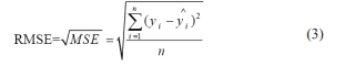
In the above expression, y1 ,y2 ,....yn are instances of response values in the dataset, y1 ,y2 ,....yn are predicted values and n is the total number of points in the dataset. If the error with respect to this subset is not acceptable, the training may be repeated. Indeed, this test is critical to insure that the network has successfully learned the correct functional relationship within the whole set of data.
The maximum relative displacements of each story for each data set scenario base on their epoch, which is a measure of the number of times all of the training vectors are used once to update the weights, are plotted in the Figs. 4and 5. RMSEs calculated for each scenario are plotted in the Figures. 6 and 7.
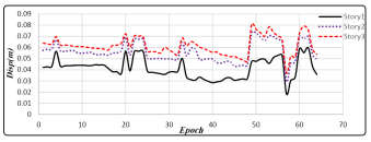
Figure 2: The maximum relative displacements of each story for 55 scenarios
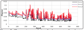
Figure 3: The maximum relative displacements of each story for 800 scenarios
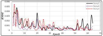
Figure 4: RMSEs calculated for 64 scenarios for train data set
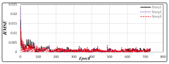
Figure 5: RMSEs calculated for 800 scenarios for train data set
As it has been shown, the very small RMSE means that the ANN model is trained on base on data set. Thereafter, the trained data is able to determine the location of damages in columns and check whether the structure is reliable or not. In this regard, 20 different random data as a test data. The performance of ANN model is checked for these data sets in the Figures 8 and 9. Moreover, the final RMSEs for the whole of trained and test data for 64 and 729 scenarios are presented in Table 1.
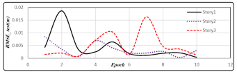
Figure 6: RMSEs calculated for 64 scenarios for random data set
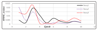
Figure 7: RMSEs calculated for 729 scenarios for random data set
Table 1: Final RMSEs for train and random data sets for each scenario| Story | 64 Scenarios | Scenarios | ||
|---|---|---|---|---|
| RMSE | RMSE_TEST | RMSE | RMSE_TEST | |
| 1 | 0.006 | 0.0104 | 0.01 | 0.014 |
| 2 | 0.003 | 0.007 | 0.016 | 0.011 |
| 3 | 0.004 | 0.017 | 0.01 | 0.01 |
With reference to the plots and final results of two different scenarios, it can be perceived that there is not much difference between these data scenarios. In other words, the trained ANN model does not care about the increment of input data. This is one of the most important benefits of ANN methods that can reduce the computational effort without any significantly decrease inaccuracy. This feature is helpful in structural damage detection as well as seismic reliability.
Linking ANN model to seismic reliability assessment
Once the ANN model is created, it will be used as a reliability method. Five random variables are considered for the purposed steel structure; namely, columns’ areas of first, second and third floor, elasticity modulus and gravity loads. The distribution, lower and upper bound, of each random variable are selected based on Ref. and are shown in Table 2 [19,20]. All stories have the same distribution parameters, but this does not necessarily mean that all structures have the same columns’ sections. Generally speaking, the procedure in the reliability assessment is the same as damage detection with this difference that the inputs and outputs of the SONN model should be the same as Open Sees. Subsequently, the SONN model has five PEs related to each random variables in the input layer and three PEs corresponding to the maximum relative displacement of each story in the output layer. This procedure is, exactly the same as before, performed through the interaction between MATLAB and Open Sees-a network and a finite element model, Figure. 10.
Table 2: Statistical Distribution and Moments of Random Variables
| Random Variables | Distribution | Mean | Gravity Loads |
|---|---|---|---|
| Columns’ Sections | Normal | 25 cm2 | 2.5cm2 |
| Elasticity Modulus | Normal | 2x10¹¹kN/m2 | 2x10⁹ kN/m2 |
| Gravity Loads | Normal | 50kN | 10kN |
The failure probability for each number of iteration is obtained by MCS Table3.The failure probability is the likelihood of passing through the Immediate Occupancy limit state (IO), which is equal to maximum relative displacement of 1%.Although MCS can calculate the failure probability readily, it can achieve to acceptable accuracy in high number of iterations. In other words, the failure probability in the high number of iterations is time-consuming and sometimes MCS is not applicable for complicated structures, such as airplane, helicopter, bridge, and so forth. Therefore, in these cases, ANN models can help MCS have a decent accuracy in the failure probability estimation. With reference to Table 4, the ANN model is trained by MCS. In fact a certain number?1000 in this study?training pairs is needed to train the network. The training data can be obtained by Shannon Information Entropy simulation with a certain number of iteration. Afterward, the ANN learns this process and try to imitate the relation between input and output data. Therefore, a combination of ANN and Shannon Information Entropy simulation with only a certain iteration can take the place of Shannon Information Entropy simulation in the large number of iterations and address the problem of timeconsuming in Shannon Information Entropy simulation although this replacement has an approximation.
In this study the number of training pairs and the network is which trained by 1000 training data is called ANN1000.
The ANN accuracy is acceptable after 1000 iterations (here, which is named ANN1000 model). The failure probability for each iteration is calculated by the ANN1000 model. Owing to RMSE, the ANN1000 model works accurately. This model can be applied to calculate the failure probability for any arbitrary iteration number that MCS could not be applied (for instance, the failure probability for 10000 iterations in this case).
Conclusions
In this study, an artificial neural network approach is employed to determine the quantification and location of damages in the columns. In addition to damage detection, the SONN model can evaluate the failure probability after training. The SONN model is successfully connected to Shannon Information Entropy simulation in order to reduce the computational effort required for reliability analysis of complicated structures to an acceptable level. In other words, the SONN model learns and imitates the relation between inputs and outputs. The SONN -based Shannon Information Entropy simulation method is more accurate than the SONN -based response surface and polynomial-based methods that were done in past studies. Additionally, this research has shown the capacity of this method in substitution of every other method with high accuracy. It has shown that the SONN model, which is trained after only1000 iterations can calculate the failure probability for any arbitrary iteration number. Although in this research 1000 iterations, this value can increase according to the complexity of the problem and required accuracy, and this limit can be determined by assorted methods such as RMSE. This approach can be applied to the realistic models with implicit limit state functions. Furthermore, the application of this approach for large structures and infrastructures reduces time and computational efforts [21-31].
References
- MI Friswell, JET Penny (1992) “A simple nonlinear model of a cracked beam,” in Proceedings of the International Modal Analysis Conference
- OS Salawu (1997) “Detection of structural damage through changes in frequency: a review,” Eng. Struct 19:
- E Ozkaya, HR Oz (2002) “Determination of natural frequencies and stability regions of axially moving beams using artificial neural networks method,” J. Sound Vib 252: 782-
- S Suresh, SN Omkar, R Ganguli, V Mani (2004) “Identification of crack location and depth in a cantilever beam using a modular neural network approach,” Smart Mater. Struct 13:
- A Bakhshi, SM Vazirizade (2015) “Structural Health Monitoring by Using Artificial Neural Networks,” in 7th International Conference of Seismology and Earthquake Engineering
- HM Gomes, AM (2004) Awruch, “Comparison of response surface and neural network with other methods for structural reliability analysis,” Struct. Saf 26:
- C Bucher, T Most (2008) “A comparison of approximate response functions in structural reliability analysis,” Probabilistic Eng. Mech
- AH Elhewy, E Mesbahi, Y Pu (2006) “Reliability analysis of structures using neural network method,” Probabilistic Mech 21:
- XL Guan, RE Melchers (2001) “Effect of response surface parameter variation on structural reliability estimates,” Saf 23:
- J Cheng, RC Xiao (2005) “Serviceability reliability analysis of cable-stayed bridges,” Struct. Eng. Mech 20:
- J Zhang, RO Foschi (2004) “Performance-based design and seismic reliability analysis using designed experiments and neural networks,” Probabilistic Eng. Mech 19:
- T Most (2005) “Approximation of complex nonlinear functions by means of neural networks,” Weimarer ptimierungs-und Stochastiktage 2:
- MT Hagan, HB Demuth, M H Beale (1996) Neural network design. Pws Pub.
- H Demuth, M Beale (1993) “Neural network toolbox for use with
- SS Haykin (2009) Neural networks and learning machines, vol. 3. New York: Prentice
- CM Bishop (1995) Neural Networks for Pattern Oxford University Press,
- S Mazzoni, F McKenna, MH Scott, GL Fenves (2006) “OpenSees command language manual,” Pacific Eng. Res.
- M Niazi, H Kanamori (1981) “Source parameters of 1978 Tabas and 1979 Qainat, Iran, earthquakes from long-period surface waves,” Bull. Seismol. Soc. Am
- S Mahadevan, A Haldar (2000) Probability, reliability and statistical method in engineering design. John Wiley &
- DG Lu, PY Song, XH Yu (2014) “Analysis of global reliability of structures,” in Safety, Reliability, Risk and Life-Cycle Performance of Structures and Infrastructures, CRC Press
- J Mahmoudi, MA, Arjomand M Rezaei, MH Mohammadi (2016) “Predicting the Earthquake Magnitude Using the Multilayer Perceptron Neural Network with Two Hidden Layers,” Civil Engineering Journal, January 2:
- Alexander (1992) Identification of Earthquakes and Explosions Using pattern Recognition Techniques on Frequency- Slowness seismic Images. EOS
- Allamehzadeh, M, P Nassery (1997) Seismic Discrimination Using a Fuzzy Discriminator, Pajouheshnameh, IIEES, Tehran.
- Allamehzadeh M (1999) Seismic Source Identification Using Self-Organizing Technique, 3th International Conference on Seismology & Earthquake Engineering. 17-19 May,
- S Haykin (1999) “Neural networks; a comprehensive foundation,” second
- MJD Powell (1987) Radial basis functions for multivariable interpolation: a review, In J. C. Mason and M. G. Cox, editors, Algorithm for Approximation. Clarendon Press,
- DS Broomhead, David Lowe (1988) “Multivariable Functional Interpolation and Adaptive Networks,” Complex Systems Publications,
- T Poggio, F Girosi (1990a) “Extension of a theory of networks for approximation and learning: dimensionally reduction and clustering,” In Proceeding Image Understanding Workshop Pittsburgh, Pennsylvania, Morgan Kaufmann
- Der ZA, AC Less (1985) Methodologies for Estimating t (f) from short- period Body Waves and Regional variations of t (f) in United states. Geophys. J
- Burger RW, T Lay, LJ Burdick (1987) Average Q and yield Estimates from the pahute Mesa test site. Bull. Seism. Am 77:
- Rundle JB, Turcotte DL, Donnellan A, Grant-Ludwig L, Gong G (2016) Nowcasting earthquakes. Earth and Space Science 3:
- Sarlis NV, Skordas ES, Varotsos PA (2011) The change of the entropy in natural time under time-reversal in the Olami- Feder-Christensen earthquake model. Tectonophysics, 513: 49-53.