Journal of Engineering and Applied Sciences Technology

Introduction

Geo-electrical resistivity survey is a technique used in a wide range of geophysical investigations which include characterization of aquifer, geo-electrical imaging, mineral exploration, borehole investigation, archaeological surveying, geological mapping [1]. It involves the detection of the surface effects produced by the electric current in the subsurface. Electrical methods are generally classified according to the energy source involved, which could be natural or artificial methods [2]. Electrical resistivity technique is an effective tool in delineating areas of good potential for groundwater development [3].

Aquifers in geological terms are referred to as bodies of saturated rocks or geological formations through which volumes of water find its way into wells and springs. Aquifers are characterized by petro-physical properties such as hydraulic conductivity, transmissivity and storage coefficient. The characterization of aquifers could be done using certain geophysical techniques like electrical resistivity, electromagnetic induction, ground penetrating radar (GPR) and seismic techniques [4]. An aquifer is described by its depth, thickness, transmissivity and hydraulic conductivity through the process of recharge and discharge via water cycle [5].

Vertical electrical sounding (VES) is a geophysical technique that uses direct current to determine subsurface resistivity. The main objective of vertical electrical sounding (VES) is to observe vertical variation of resistivity with depth in the subsurface. It is the best technique adopted for aquifer characterization, resistivity and depth determination for aquifer and flat lying layered rock structures etc. Vertical Electrical Soundings (VES) technique has proved to be widely or mostly used in aquifer characterization studies due to its simplicity. Using this technique, resistivity, thickness and depth of aquifers or subsurface layers and their groundwater yielding capacities can be inferred [6].

Area of Study

The area of study (Kaani) is located in Khana Local Government Area of Rivers State, Southern Nigeria within the Tropical Rain forest zone as shown in Figure 1. It lies between latitude 4.67608°N and 4.7101N° and longitude 7.3619°E and 7.36153E° with an elevation of 16m and 19m respectively [7]. The area covers about 49,631.54hackers of land with a rainfall pattern that is in a bimodal form which usually start effectively from late February to October with a period of low precipitation in August commonly called August break. The period of effective low precipitation occurs mainly from late November to early March.

The average rainfall in the study area is between 2000mm to 2500mm with monthly temperature range of 26°C to 35°C and relative humidity varying from 81% to 87% which is dependent on the season (rainy season and dry season) [7].

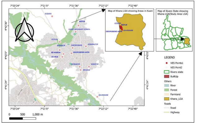
Figure 1: Map Showing the Study Area

Materials and Methods Materials

Materials used for this study include Herojat resistivity meter, Global Positioning System (GPS), pairs of electrodes (current and potential electrodes), measuring tape, hammers, reels of cables (wires) and writing materials (pen and paper).

Method
Procedure for Field Data Acquisition

The vertical electrical sounding (VES) point were mapped out using the global positioning system (GPS), direct current (DC) was introduced into the ground by means of Herojat resistivity meter through the current electrodes and the resulting potential difference across the potential electrodes was measured with respect to the current electrodes.

The procedure is based on the fact that as the spacing or distance between the current electrodes increases, current penetrates continuously deeper into the ground. The current electrodes are symmetrically moved outwards whereas the potential electrodes are kept at a fixed spacing until the observed potential difference becomes too small to be measured before being moved outward to a new spacing. This implies that the potential electrodes are changed after a number of changes in the current electrodes.

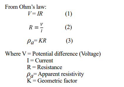
At each electrode spacing, the values of the current and potential difference are measured and recorded as well as the geometry value. The value of the resistance is computed by dividing the potential difference (voltage) by the current (eqn. 2) and the apparent resistivity is obtained by the multiplication of the computed resistance value and the geometric factor (eqn. 3) for the electrode spacing used.

Vertical Electrical Sounding (VES) measurements are made by driving an array of current and potential electrodes into the ground, at set probe spacing. This creates an electric field allowing for the measurement of the potential and hence the calculation of the electrical resistance.

In the field, the procedure is to determine a fixed point or centre and the spreading distance and electrode configuration to be used, this is to allow for equal spread on the survey area. The greater the electrode spacing, the deeper the current will penetrate into an inhomogeneous earth and the resistivity so measured does not represent the true resistivity of the subsurface, it is the apparent resistivity because of the inhomogeneity of the subsurface [8].

Vertical Electrical Sounding (VES) Curve

The computer software IPI2Win was used to plot a graph of apparent resistivity against the half current electrode spread AB/2, for both the interpretation of the vertical electrical sounding (VES) data and generation of VES curves types. These curves type vary from station to station based on the geology of the area and also provides an insight on the number of geo-electric layers in each VES station as shown in Figures 2-5.

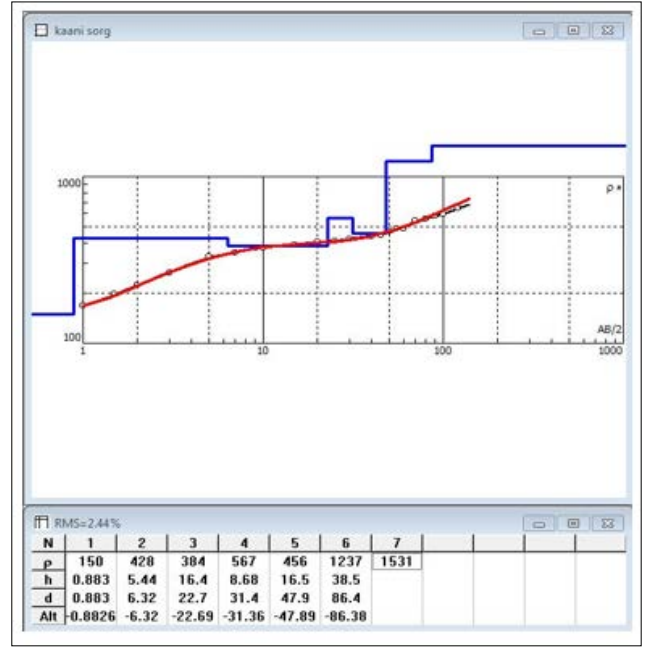
Figure 2: VES Curve for Bekue - Station 1

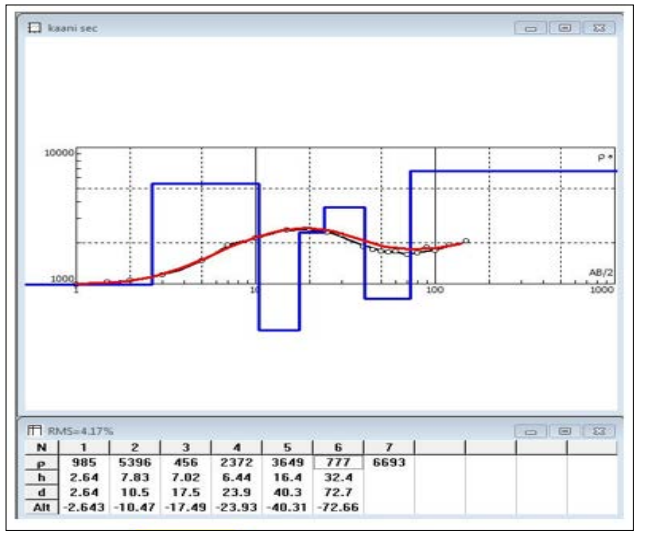
Figure 3: VES Curve for Kaani - Station 2

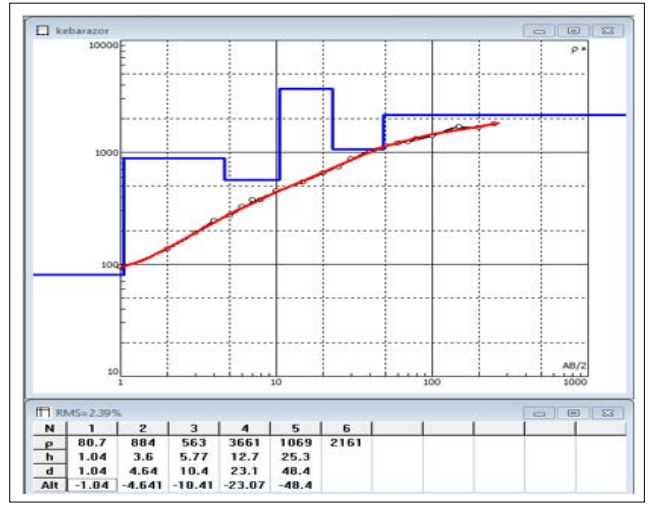
Figure 4: VES Curve for Kebarazor - Station 3

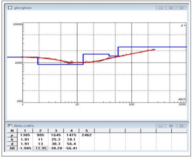
Figure 5: VES Curve for Gborgbara - Station 4

Results and Discussion

The results of the geo-electrical (vertical electrical sounding) investigation carried out in the study area are presented in Tables 1-2 for the various stations, while Figures 2-5 show the plots of computed apparent resistivity values against depth of probe for each VES station.

The VES curve of Bekue as shown in Figure 2 is a type KKH curve and revealed the presence of seven geologic layers with resistivity values ranging from 150Ωm to 1531Ωm, thickness values from 0.883m to 38.5m and depth from 0.883m to 86.4m. The last layer with resistivity value of 1531Ωm cannot be determine due to undefined thickness and depth.

The VES curve of Secondary School Kaani as shown in Figure 3 is a type KAK curve and revealed the presence of seven geologic layers with resistivity values ranging from 456Ωm to 6693Ωm, thickness values from 2.64m to 32.4m and depth from 2.64m to 72.7m. The resistivity values of the VES station corresponds to that of a sandstone formation.

The VES curve of Kebarazor as shown in Figure 4 is a type KK curve and indicates the presence of six geologic layers with resistivity values between 80.7Ωm and 2161Ωm, thickness values between 1.04m and 25.3m and depth values between 2.64m and 72.7m. The fifth layer of this VES station has a potential for quality

aquifer which can be transmit large volume of water.

The VES curve of Gborgbara as shown in Figure 5 is a type HK curve and reveals the presence of five geologic layered formations with resistivity values ranging from 905Ωm to 2462Ωm, thickness values from 1.91m to 18.1m and depth values from 1.91m to 56.4m. The first layer of this VES station is the topsoil with a resistivity value of 1385Ωm, thickness 1.91m and depth of 1.91m, it is a very thin layer with high resistivity value. The fourth layer of has the characteristics of a good aquifer which can be transmit large volume of water to borehole.

Table 1: Summary of Vertical Electrical Sounding Parameters

Table 2: Summary of Aquifer Parameter at Different VES Station

Conclusion

From the analysis and interpretation of the results of Vertical Electrical Sounding (VES) carried out in the study area, the following conclusions were reached:

• The resistivity value of aquifer in the study area ranges from 61.75Ωm to 7487 Ωm, the thickness value of the aquifer in the study area ranges from 0.88m to 55.85m and depth value of the aquifer ranges from 0.882m to 105m.

• The interpreted vertical electrical sounding curve revealed the following curve types KK, AH, HK, KKH, HK, QKK and QKAK.
• The hydraulic parameter which are (hydraulic conductivity, transmissivity and storativity) of the aquifer in the study area was The hydraulic conductivity value of the aquifer in the study area ranges from 0.000217 to 0.0311m/day, the transmissivity value of the aquifer in the study area ranges from 1.3719 to 17.888Ωm2 and the storativity value of the aquifer in the study area ranges from 1.32x10-5 to 9.21x10-6
• Dar-zarrouk parameter which are (transverse resistance and longitudinal conductance) of the aquifer in the study area was obtained. The transverse resistance value of the aquifer in the study area ranges from 6 to 74710 and the longitudinal conductance value in the study area ranges from 0.00217 to 0.0311Ω-1. The result obtained in the study can be use in siting of water well to avoid borehole failure in the study area.

References

1. Amakiri ARC, Amoniaeh J, Otugo VN (2024) Estimation Electrical Formation Factor and Porosity from VES for the Aquifers in Part of Bayelsa State, Nigeria. International of multidisciplinary research and growth evaluation 5: 480-487.
2. Jatau BS, Patrick NO, Baba A, Fadele SI (2013) The Use of Vertical Electrical Sounding (VES) for Subsurface Geophysical Investigation around Bomo Area, kaduna State, IOSR Journal of Engineering (IOSRJEN) 3: 10-15.
3. Onimisi M, Daniel A, Kolawole MS (2013) Vertical Electrical Sounding Investigation for Delineation of Geoelectric Layers and Evaluation of Groundwater Potential in Ajagba, Asa and Ikonofin Localities of Ola Oluwa Local Government Area of Osun State, South Western Nigeria. Research Journal of Applied Sciences, Engineering and Technology 6: 3324-3331.
4. Salako AO, Adepelumi AA (2018) Aquifer Classification and Characterization. Groundwater for Sustainability Development 15.
5. Onyenweife GI, Nwozor KK, Onuba LN, Nwike IS, Egbunike ME (2020) Estimation of Aquifer Parameters in Awka and Environs, Anambra State, Nigeria, using Electrical Resistivity International Journal of Innovative Scientific and Engineering Technologies Research 8: 1-29.
6. Kearey P, Brooks M, Hill I (2002) An Introduction to Geophysical Third Edition, Blackwell Science Ltd 184-190.
7. Peter KD, Umweni AS (2020) Characterization and classification of soils developed from coastal plain sands and alluvium in Khana Local Government Area of Rivers State, Southern Direct Research Journal of Agriculture and Food Science 8: 246-256.
8. Telford WM, Geldart LP, Sheriff RE (1990) Applied Geophysics, Second Edition. Cambridge University Press, New York 535-539.