Limiting Heating & Cooling Peak Loads For Net Zero Carbon Buildings

Author(s): Esam Elsarrag* and Jon Nuttall

Abstract

Introduction

The research community has paid close attention to the use of MPC (Model Predictive Control Techniques) strategies in building automation and control systems (BACS) [1]. To achieve high energy and comfort performance levels, it is necessary to incorporate renewable energy generation, innovative technical system solutions (such as heat pumps), and energy storage systems. MPC is frequently used in the construction industry to forecast dynamic system behaviour in the future and have the controller alter response in accordance, resulting in energy and cost savings while ensuring thermal comfort [1-4].

The effects of the cut-off temperature and the size of the heat pump on the annual energy performance of a hybrid heating system for residential buildings were investigated by [5-6]. In order to shift the peak load and lower cooling energy usage, assess a thermal energy storage (TES) system combined with an active insulation system (AIS) to create a TES + AIS integrated wall system [7]. Results revealed that depending on the climatic circumstances, different minimum system sizes are required to obtain energy savings. Phase change materials (PCMs) were suggested by Osterman as a TES system to lower the amount of energy used for cooling and heating in an office building [8]. It was discovered that from May to September, 58 kWh of cooling energy can be saved, and from October to April, 84 kWh of heating energy can be saved. A parametric analysis and design optimization of an active TES system for space cooling was also carried out by [9]. Similar to this, Stritih & Butala suggested an experimental TES system for cooling buildings that resulted in energy savings ranging from 14% to 87% on average [10]. Peak load shifting has also been studied in the past.

Using observed data and simulation results, Yin, et al., assessed and optimised the effects of pre-cooling and TES in commercial buildings [11]. They saw a 15% to 30% drop in peak-time electricity use. The impacts of building mass, utility rate, thermal comfort, central plant capabilities, and economizer on the effectiveness of demand limiting management using the building thermal mass and active thermal storage were also investigated by Zhou, et al., using parametric analysis [12]. An interior room temperature resetting technique was used by P Xu, et al., in a site study to lower the daily peak demand in a medium-weight building [13]. According to this plan, zone temperatures are kept at the lower thermal comfort level during off-peak hours and are reset to the upper thermal comfort limit during peak hours. to improve the applicability of the building zone temperature set-point. By changing the regulation of the heating, ventilation, and air-conditioning (HVAC) system, P Xu, et al., demonstrated the potential to reduce peak electrical demand in moderate-weight commercial buildings [14].

Field studies revealed that during peak hours, the chiller power was lowered by 80-100% (1-2.3 W/ft2) without resulting in concerns about thermal comfort. The use of building thermal mass for shifting and reducing peak cooling loads in commercial buildings has been widely researched, according to Braun, who also offered particular results from simulations, laboratory experiments, and field surveys [15].

There has also been studies regarding predicting the loads. The optimal forecast of external temperature and thermal load has been taken into account by D’Ettorre, et al., when investigating the optimal control problem using mixed-integer linear programming (i.e. model predictive control) [16]. They illustrate achievable cost savings as a function of both prediction horizon and storage capacity in a dimensionless manner in comparison to a conventional rule-based control technique with no storage. L Xu, et al., proposed a load-uncertainty-aware adaptive optimal peak building demand limitation approach for a month [17]. In this study, the probabilistic building demand profiles are predicted using a probabilistic load forecasting model. Seasonal case studies are chosen for an educational structure in Hong Kong. The established demand limitation method is validated by real-time case studies. The monthly demand limiting threshold optimization, the probabilistic load forecasting model, the calculation of the economic benefit and success likelihood of a demand limiting control, and the outcomes of the real-world case studies are all covered in this paper.

However, a problem with the aforementioned studies is that they mainly focus on systems that are energy efficient or for reducing loads as well as predictive systems for dynamic loads. This paper places emphasis on reducing thermal loads and not electrical loads in order to utilise thermal systems with less needed capacities as a result. Weather data is becoming a crucial part of almost every new building design and significant renovation due to the rising need for more sustainable and energy-efficient buildings and services to address climate change. To conduct simulations using the ApacheSim technique in VE Compliance, the CIBSE weather files Test Reference Year (TRY) & Design Summer Year (DSY) datasets are necessary. For every hour of the year, these weather files in IESVE contain information on factors including dry bulb and wet bulb temperatures, wind speed and direction, solar height and azimuth, cloud cover, etc. In order to understand the effects of various load estimate parameters on heating and cooling loads, dynamic simulation is utilised in this study to forecast the peak heating and cooling loads for an office building. Peak loads’ response to weather information, heat gains, and shade have also been evaluated.

Simulation Weather Files

With the increasing demand for more sustainable and energyefficient buildings and services to combat climate change, weather data has now become an essential component of virtually every new building design and major refurbishment. CIBSE weather files Test Reference Year (TRY) & Design Summer Year (DSY) datasets are required to run simulations using ApacheSim method in VE Compliance. These weather files in IESVE contain data for variables including dry bulb & wet bulb temperature, wind speed & direction, solar altitude & azimuth, cloud cover etc for each hour of the year. The new National Calculation Modelling (NCM) Guide came into force on 15 June 2022. It includes several important changes, including an upgrade to the 2016 CIBSE Test Reference Year (TRY) weather data sets.

Along with the use of the 2016 CIBSE Weather Data files, Dynamic Simulation Model software must also meet or exceed the classification of dynamic modelling under CIBSE AM11: Building performance modelling. Additionally, the new guidance refers to CIBSE Guide A: Environmental design. The weather variables are synthesised into 2 types of CIBSE weather files are the Design Summer Year (DSY) and the Test Reference Year (TRY).

The TRY weather file represents a typical year and is used to determine average energy usage within buildings. The weather file consists of average months selected from a historical baseline. The standardised methodology selects the representative months using air temperature, relative humidity, and cloud cover (as a proxy for global solar irradiation) with wind speed as a secondary parameter. The primary variables are used to find the three months with the lowest ranking. From these months, the month with the most average wind speed is then chosen as the representative month for that location. TRYs are available for 14 locations across the UK. The TRY is used for energy analysis and for compliance with the UK Building Regulations (Part L).

The DSY represents warmer than typical year and is used to evaluate overheating risk within buildings. The updated DSY methodology is based on that used in CIBSE TM49, which used a new metric to define the level of overheating. Three metrics are used to define overheating, these are defined first and then are used to rank and select suitable years for all 14 locations.

However, the standard simulation weather files are sourced from various places and converted into the standard FWT file format. Usually, the FWT will have an abbreviation that points out where the data was acquired e.g., EWY = Example Weather Year. These are individual weather years sourced from the MET office.

Figure 1 presents the hourly profile in summer for dry bulb temperature and solar radiation. The EWY weather file (e.g., London) has lower temperature in winter whilst the TRY has higher temperature in Summer. The variation between weather data suggests a deviation in load estimates. For building regulations, engineers are required to ensure weather files TRY and DSY are up to date.

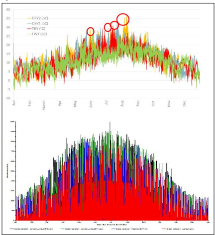
Figure 1: EWT TRY & DSY Weather Files Comparison - DBT and Global Radiation

Limiting Peaks in Heating Loads

Dynamic simulation modelling using IESVE is employed for an office building. NABERS profile are applied to provide annual and peak heating loads using different scenarios e.g. with and without considering interna heat gains and variation of weather files as detailed in Table 1.

As shown in Table 1 below, different scenarios are conducted to understand the impact of the heat gains and temperature set points within occupied a non-occupied period.

The annual and peak loads simulation results for different scenarios, as presented in Table 1, are depicted graphically in Figure 2 below for TRY and EWY weather files. The followings have been pointed:

? The simulation results showed high discrepancy between TRY and EWY weather files for peak l loads prediction scenarios (typical value < 20%).
? For any specific scenario, irrespective to weather file used, the peak load varies when considering diversity in internal gains with a typical value of 10% which is an obvious result, however, this has shown small impact on the annual heating demand prediction.

Unlikely, NABERS profile showed high spikes for peak heating loads which suggests further analysis to align with NZC roadmap. Figures 3 and 4 below show the impact of temperature control on the peak with or without considering internal heat gains. The NABERS Profile 8am to 6pm (21°C Occupied/OFF Non occupied) showed a higher peak compared to the hybrid profile NABERS 8am to 6pm (Ramp Function of 21°C Occupied/ 19°C Non occupied between 7pm to 7am).

he later showed comparable or less annual energy demand as well. This is due to the fact that the building loses heat during night hence higher peaks are required in the morning. The overnight set will just compensate such losses resulting a comparable annual demand i.e., reducing the peak in the morning without comprising the annual heating demand. The peak loads also showed 50% reduction of NABERS 21°C if a ramp function is applied- NABERS 19-21°C.

The study suggests that for NZC design, there is an opportunity to lowering peak days if 20°C is set which will result in dramatic reduction, but certainly this will require further thermal comfort analysis.CIBSE loads generated by IESVE need to be further analysed in detail to understand the discrepancies properly.

Table 1: Heating Load Simulation Scenarios

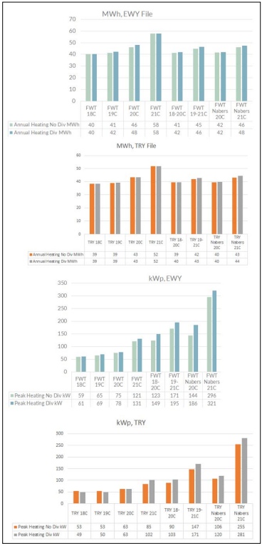
Figure 2: Annual and Peak Loads for Different Simulation Scenarios Using EWT and TRY Weather Files

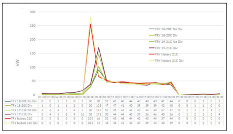
Figure 3: Peak Load Shrinking Scenarios

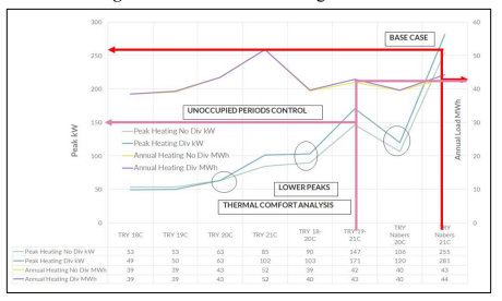
Figure 4: Impact of Temperature Control on Annual and Peak Loads

Limiting Peak Cooling Loads

DSM is implemented using NABERS profile to provide annual and peak cooling loads. Different scenarios are assessed e.g., with and without considering shading from adjacent properties and the impact of different weather files as detailed in Table 2 below.

As shown in Table 2 below, different scenarios are conducted to understand the impact of the heat gains and the shading of adjacent properties with the variation of weather files.

Table 2: Cooling Load Simulation Scenarios

Figure 6 demonstrates the impact of internal heat gains diversity and shading of adjacent properties on the cooling loads. The followings have been observed: Regardless to weather file used in the simulation, shading of adjacent property have a big impact on cooling load calculations resulting in parallel lines. Depends on the glazing ratio, internal gains in this study showed 2% impact on cooling load whilst the combination of both showed 16%. As depicted graphically, the impact of shading of adjacent property can impact the cooling load, in average, by 10%. This suggests careful attention in cooling loads calculations considering future planning.

As shown in Figure 5, the variation between peaks generated from EWT, TRY, DSY1 & DSY2 weather files. DSY2 will provide higher peak, however, the noon time peaks remain consistent for all weather files except for the DSY1 remained the highest during the day.

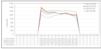
Figure 5: Variation of Peak with the Weather File

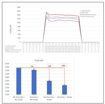
Figure 6: Impact of Gains and Shading on Peak Load

As shown in Figure 7, interestingly, although peak loads vary dramatically between EWY & TRY weather files, but the annual cooling loads remained unchanged. The variation in peak loads between DSY2 and DSY1 weather files remained within 8% and between DSY2 and TRY is about 13% for all typical cases.

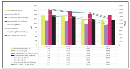
Figure 7: Peak and Annual Cooling Loads All Scenarios

It is worth noting that for peak load calculations, in this study the external shading can offset the variations between DSY and TRY weather files i.e., DSY sim results + Shade is approximately equal to the TRY sim results without shade, see Figure 8. This suggests engineers’ attention to simulation results when comparing load calculations.

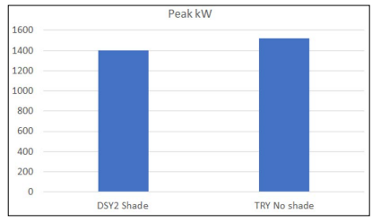
Figure 8: Impact of Shading on Peak Load Analysis

Conclusions

Dynamic simulation is used to predict the peak heating and cooling loads for an office building to understand the impact of different load estimate parameters on heating and cooling loads.

This report discussed the impact of using different weather files, heat gains and shading on the peak loads. It also provided guidance to minimise heat peak loads spikes.

In summary: ? NABERS profile showed high spikes for peak heating loads, but the use of over night control reduced dramatically the peak heating load by 50% without comprising the annual heating demand.
? There is an opportunity to dramatically lowering further the peak days if 20°C is used as set but thermal comfort analysis is required.
? Shading of adjacent property have a big impact on cooling load calculations which depend on the glazing ratio. In this study, it exceeded 10% which suggests careful attention in cooling loads calculations whilst considering future planning

References

1. Serale G, Fiorentini M, Capozzoli A, Bernardini D, Bemporad A, et al. (2018) Model Predictive Control (MPC) for Enhancing Building and HVAC System Energy Efficiency: Problem Formulation, Applications and Opportunities. Energies 11: 631.
2. Elsarrag E, Alhorr Y (2012) Modelling the thermal energy demand of a Passive-House in the Gulf Region. International Journal of Sustainable Built Environment 1: 1-15.
3. Hazyuk I, Ghiaus C, Penhouet D (2014) Model Predictive Control of thermal comfort as a benchmark for controller performance. Automation in Construction 43: 98-109.
4. Elsarrag E, Alhorr Y (2017) Towards near zero energy home. In: Energy Efficient Buildings. Eng Hwa Yap, Intech Open, Book 1-214.
5. Bagarella G, Lazzarin R, Noro M (2016) Sizing strategy of on-off and modulating heat pump systems based on annual energy analysis. International Journal of Refrigeration 65: 183-193.
6. Bianco V, Scarpa F, Tagliafico L A (2017) Estimation of primary energy savings by using heat pumps for heating purposes in the residential sector. Applied Thermal Engineering 114: 938-947.
7. Jung S, Yoon Y, Im P, Salonvaara M, Dong J, et al. (2022) Peak cooling load shift capability of a thermal energy storage system integrated with an active insulation system in US climate zones. Energy and Buildings 277: 112484.
8. Osterman E, Butala V, Stritih U (2015) PCM thermal storage system for ‘free’ heating and cooling of buildings. Energy and Buildings 106: 125-133.
9. Ru?evskis S, Akishin P, Korjakins A (2020) Parametric analysis and design optimisation of PCM thermal energy storage system for space cooling of buildings. Energy and Buildings 224: 110288.
10. Stritih U, Butala V (2011) Energy savings in building with a PCM free cooling system. Strojniski Vestnik/Journal of Mechanical Engineering 57: 125-134.
11. Yin R, Xu P, Piette M A, Kiliccote S (2010) Study on AutoDR and pre-cooling of commercial buildings with thermal mass in California. Energy and Buildings 42: 967-975.
12. Zhou G, Krarti M, Henze G P (2008) Parametric analysis of active and passive building thermal storage utilization. International Solar Energy Conference 193-203.
13. Xu P, Haves P, Piette M, Zagreus L (2005) Demand shifting with thermal mass in large commercial buildings: Field tests, simulation and audits 11: 1-80.
14. Xu P, Haves P, Piette M A, Braun J E (2004) Peak Demand Reduction from Pre-Cooling with Zone Temperature Reset in an Office Building. Aceee 376-386.
15. Braun J E (2003) Load control using building thermal mass. Journal of Solar Energy Engineering,Transactions of the ASME 125: 292-301.
16. D’Ettorre F, Conti P, Schito E, Testi D (2019) Model predictive control of a hybrid heat pump system and impact of the prediction horizon on cost-saving potential and optimal storage capacity. Applied Thermal Engineering 148: 524-535.
17. Xu L, Wang S, Xiao F (2019) An adaptive optimal monthly peak building demand limiting strategy considering load uncertainty. Applied Energy 253: 113582.

Our Pubmed Indexed Articles