Author(s): <p>Aamod Shanker* and Girish Nivarti</p>
The differential equations underlying the non-linear dynamics of turbulent fluid flow are extended to the transport of optical energy and optical phase in coherent lasers in a new theoretical framework. Since light acts like a pure, incompressible, inviscid fluid, the momentum and mass transport of the Navier-Stokes equations translate directly to the intensity and phase transport equations in scalar diffraction theory, respectively. The non-linear term in the phase transport equation describes the emergence of turbulent dynamics near cusps and singularities in the optical field, enabling insights into the topology and dynamics of turbulence/speckle in 6D phase space. A better understanding of the mathematical forms of turbulent wave dynamics allows for reformulating the inverse computational problem for the perennial and current problems in the physics and engineering - imaging through turbulent media, understanding stochastic effects in sub 20nm extreme ultraviolet lithography for extending Moore’s law, holographic reconstruction of chaotic diffusion in image processing - but in context of latest computational and sensing capabilities. Turbulence in visible laser light can be easily measured with inexpensive table-top laser sources, scientific cameras, and simple imaging optics, enabling volumetric energy measurements. Combined with the most current mathematical understanding and computational tools for hydrodynamics modeling, we hope to usher in a new understanding of super-linear dynamics in natural flow processes
Light is a super fluid, with no rest mass (latin root ”light” for weightlessness), as well as no stickiness or viscosity characteristic of shear stress in fluid mechanics. Hence, the wave mechanics of light propagation encompasses only the inviscid aspect of fluid dynamics, allowing for a simplification of the laws of fluid mechanics in their differential form to describe the laws of optical propagation. Local descriptions of optical dynamics with partial differential equations (PDEs) parallel the Navier-Stokes equations, where the optical intensity plays the role of fluid mass, and the optical phase is the fluid momentum, guiding the propagation of mass. Additionally since there is no viscosity, the laws of optical propagation are isomorphic to the Euler equation, the inviscid form of the Navier-Stokes equation for flow.
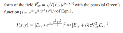
Due to its low viscosity or high Reynolds number (R), coherent light enters turbulent regimes of flow rapidly due to even slight disturbances, causing laser beams to eventually develop granular stochastics called ’speckle’ - essentially turbulent light. The mathematical model starts with the fundamental differential equation of electric field propagation (Helmholtz equation), which models light as a diffusion process in x-y, with propagation in the z direction with temporal frequency ω, such that Ex;y;z;t = Ex;yeikz+iwt , then

is the effective diffusion Laplacian with a preferential direction of propagation (z);

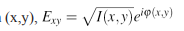
is the dispersion relation, linear for light; c is the speed of light. The electric field is often represented as a complex valued vector at each (x,y),
by splitting into two variables I and φ that are conjugates of each other, the dynamics of the equation alternates between the two at each propagation step. Here I is the optical intensity, analogous to the mass density of a fluid is analogous to the fluid velocity vector ~v representing the local direction and velocity of energy flow in fluids, or equivalently of phase gradients in light (Huygen’s principle). The differential equations of fluid flow consist of mass (p) and momentum(pv) transport; the mass transport equation for fluid is the continuity equation and can be directly compared to the transport of intensity equation for light, for fluid ,
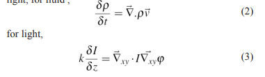
The Transport of Intensity Equation, or TIE (Eqn. 3)is isomorphic with the continuity equation of fluid transport (Eqn. 2). It is derived from the Helmholtz equation (Eqn. 1) by convolving the eikonal
The paraxial approximation assumes all third order derivatives, as well as non-linear terms in phase or intensity to be negligibly small, yielding the intensity transport equation 3. The transport of intensity can be expanded as linear in both intensity I and phase φ, the first and second terms corresponding to focusing by parabolic surfaces and bending by a prism, respectively. The non-linear, turbulent terms arise in the momentum transport equation, also called the Navier Stokes equation (where p is the fluid pressure),

For irrotational flow, substitute here φ is a scalar potential, to get the equation of a streamline (Eqn. 6). For light, the equivalent equation of momentum transport is the transport of phase equation obtained from the imaginary part of the Helmholtz eqn (Eqn. 1) with the eikonal form of or by taking the argument of the Green’s function convolution (Eqn. 4) to get Eqn. 7, the phase transport
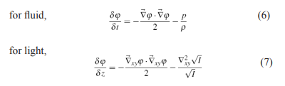
which describe the momentum or phase transport of fluid and light respectively. The first non-linear term (φ)2 is the Bernoulli flow along a streamline, the second term is the pressure along the streamline. Interestingly, the curvature of the electric field amplitude acts as optical pressure, causing phase to evolve locally near regions of amplitude curvature. The level sets of this second non-linear term are the positions of the zero crossing of the electric field, where both and go to infinity (Fig. 2b). This suggests a Bernoulli’s law for free space light propagation - the same way pressure is the inverse of flow speed, allowing airplanes to have lift with larger wing curvature on the top than the bottom, areas in an optical field with large phase flux (red lines in Fig. 2b) have a low pressure, causing energy to be suctioned towards cusps and singularities; much like the role of gravity in general relativity.
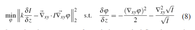
The Eqns.3,7 and Eqns. 2,6 demonstrating onset of turbulence in light and fluids respectively, are simulated in fluids and measured in light (Figs 1, 2). The phase φ can be retrieved from the coupled PDEs (Eqns.3,7 or 2,6) within a Hamilton-Jacobi variational formulation. The computational phase retrieval is posed as a minimization over the measured intensity transport with propagation z (Fig. 2a),with an additional constraint on the momentum transport (the Transport of Phase Equation).
Once the phase recovery for turbulent optical flow is posed as coupled PDEs - a process equivalent to unfolding manifolds in phase-space - many of the numerical and analytical tools used in the turbulence theories of modern

Figure 1: The simulated density r, velocity u and energy e = u·u /2 - P / p obtained for a homogeneous isotropic turbulent flow field with Re0 = 650. The density field is the measured intensity for light, and the velocity velocity field u = ∇? is analogous to for light, revealing singularities in the flow field.
physics (e.g. Kolmogorov) are applicable, with new understanding gained from free space experiments with light, complemented with current computational modeling and learning approaches. The applications are wide ranging - imaging through turbulent media (such as the brain, retina, stars), cosmological & relativistic fluid mechanics, magnetohydrodynamics of plasmas among others.

Figure 2: a. Coherent speckle intensity experimentally measured as a function of propagation, the camera measuring a 3D volume by stepping through defocus or with propagation; turbulence is seen to appear as two dimensional singularity manifolds in the measured 3D speckle intensity. In the inset, this equates to dark rivers (blue) permeating the bright intensity hills (orange). In the ininset,∇I ? ∇φ indicate point singularities, with each line singularity terminating at point singularities with opposite topological charge at either end. b. In negative contrast, the singularities pop (yellow) against intensity valleys (blue), a network of 1D lines in the 2D intensity terrain, the positions of singularity cusps indicating divergence or convergence of phase gradients or fluid momentum; measured intensity on the camera sensor is smooth, since cusps are swallowed when amplitude is squared.
View PDF