Author(s): Gerald C. Hsu
This article is Part 4 of the author’s linear elastic glucose behavior study, which focuses on fasting plasma glucose (FPG) component. It is the continuation of his previous three studies, Parts 1, 2, and 3, on linear elastic postprandial plasma glucose (PPG) behaviors
Here is his defined linear elastic FPG equation:
Where Weight is the input component (similar to stress) and FPG is the output component (similar to strain). The close relationship between Weight and FPG can also be found in his previous published medical papers (Reference 10)
GH.f-modulus is a newly defined coefficient to connect both weight and FPG, similar to the theory of elasticity in engineering:
Where Young’s modulus connects both stress and strain except Young’s modulus and GH.f-modulus are reciprocal to each other.
The author is able to connect this biomedical FPG equation with the basic concept of linear elasticity which involves stress and strain, along with the Young’s modulus of strength of materials in structural & mechanical engineering. He uses the collected data of daily body weight and daily FPG data from three type 2 diabetes (T2D) patients with separate severity levels of obesity and diabetes within three different time ranges. In addition, he uses an identical 8-month period of collected data for the three patients to conduct his analysis. He demonstrated once again that using GH.f-modulus, a “pseudo-linear” relationship connecting both weight and FPG exists in all three clinical cases, except the value of this coefficient depends on the individual patient’s severity level of chronic diseases, specifically obesity and diabetes.
The main objectives of this study is threefold. First, it is to offer a simpler FPG prediction equation to the patients. Second, it is to prove that similar to GH.p-modulus for PPG, the coefficient of GH.f-modulus indeed varies with the severity of chronic diseases in these clinical cases. Third, this constant coefficient of GH.f-modulus also differs from one-time range to another due to dynamic behavior, because blood is a living organic material.
The 7-month average value of each monthly M2 variables (i.e.,
GH-modulus) are 3.7, 2.6, and 1.0, and with an average measured
PPG values at 122 mg/dL, 114 md/dL, and 109 mg/dL, for Case
A, Case B, and Case C, respectively, which are ranked according
to the severity of their diabetes conditions.
In summary, the higher the M2, the higher values of both x (carbs/
sugar intake amount) and y (incremental PPG amount) become,
and the higher predicted and measured PPG values are. The key
conclusion from these three clinical observations is that the M2
values are varying based on the patients’ body conditions (liver
and pancreas), especially their diabetes severity. This is similar
to the different inorganic materials having the different Young’s
modules values, such as nylon ~3 versus steel ~200.
The article represents the author’s special interest in using mathphysical and engineering modeling methodologies to investigate various biomedical problems. The methodology and approach are a result of his specific academic background and various professional experiences prior to the start of his medical research work in 2010. Therefore, he has been trying to link his newly acquired biomedical knowledge over the past decade with his previously acquired knowledge of mathematics, physics, computer science, and engineering for over 40 years.
The human body is the most complex system he has dealt with,
which includes aerospace, navy defense, nuclear power, computers,
and semiconductors. By applying his previous acquired knowledge
to his newly found interest of medicine, he can discover many
hidden facts or truths inside the biomedical systems. Many basic
concepts, theoretical frame of thoughts, and practical modelingtechniques from his fundamental disciplines in the past can be
applied to his medical research endeavor. After all, science is based
on theory from creation and proof via evidence, and as long as
we can discover hidden truths, it does not matter which method
we use and which option we take. This is the foundation of the
GH-Method: math-physics medicine.
The author has spent four decades as a practical engineer and
understands the importance of basic concepts, sophisticated
theories, and practical equations which serve as the necessary
background of all kinds of applications. Therefore, he spent his
time and energy to investigate glucose related subjects using
variety of methods he studied in the past, including this particular
interesting stress-strain approach. On the other hand, he also
realizes the importance and urgency on helping diabetes patients
to control their glucoses. That is why, over the past few years,
he has continuously simplified his findings about diabetes and
try to derive more useful formulas and simple tools for meeting
the general public’s interest on controlling chronic diseases and
their complications to reduce their pain and probability of death.
This article is Part 4 of the author’s linear elastic glucose behavior study, which focuses on fasting plasma glucose (FPG) component. It is the continuation of his previous three studies, Parts 1, 2, and 3, on linear elastic postprandial plasma glucose (PPG) behaviors.
Here is his defined linear elastic FPG equation:
Where Weight is the input component (similar to stress) and FPG is the output component (similar to strain). The close relationship between Weight and FPG can also be found in his previous published medical papers (Reference 10).
GH.f-modulus is a newly defined coefficient to connect both weight and FPG, similar to the theory of elasticity in engineering
Where Young’s modulus connects both stress and strain except Young’s modulus and GH.f-modulus are reciprocal to each other.
The author is able to connect this biomedical FPG equation with
the basic concept of linear elasticity which involves stress and
strain, along with the Young’s modulus of strength of materials
in structural & mechanical engineering. He uses the collected
data of daily body weight and daily FPG data from three type 2
diabetes (T2D) patients with separate severity levels of obesity
and diabetes within three different time ranges. In addition, he
uses an identical 8-month period of collected data for the three
patients to conduct his analysis. He demonstrated once again that
using GH.f-modulus, a “pseudo-linear” relationship connecting
both weight and FPG exists in all three clinical cases, except the
value of this coefficient depends on the individual patient’s severity
level of chronic diseases, specifically obesity and diabetes.
The main objectives of this study is threefold. First, it is to offer
a simpler FPG prediction equation to the patients. Second, it is
to prove that similar to GH.p-modulus for PPG, the coefficient
of GH.f-modulus indeed varies with the severity of chronic
diseases in these clinical cases. Third, this constant coefficient
of GH.f-modulus also differs from one-time range to another due
to dynamic behavior, because blood is a living organic material.
Patients with varying chronic diseases would have different
coefficient of GH.f-modulus. Both Case A and Case B are longterm T2D patients; however, their weights are still within the
boundary of normal and slightly overweight with BMI around 25.
Therefore, using 14 semi-annual periods for Case A and 10 months
for Case B, their coefficients are the same at 0.67. However, due to
Case A’s stringent lifestyle management to control his diabetes, his
weight and glucoses, including FPG, have reduced significantly,
especially in 2020 where his coefficient became 0.59 in comparison
with Case B’s 0.66.
Case C is another story. His extreme-obese condition (BMI at
40.7) is much more serious than his diabetes conditions with a
4-year history. In order to compensate for his heavy weight, he
must have a lower value of the GH.f-modulus (his coefficient of
0.36 is at 54% level of 0.67 for both Case A and Case B) in order
to match with his measured FPG level (almost normal).
At first glance of this coefficient, it appears that it as a variable,
rather than a constant. However, by examining their values within
a reasonable time span, they do not vary that much. That is why it
is called a “pseudo-linear” relationship. Once we have collected
sufficient data for a particular time period, we can then easily figure
out the suitable coefficients for both FPG and PPG, i.e. GH.f-modulus
and GH.p-modulus respectively, to be used in glucose predictions.
To learn more about the author’s GH-Method: math-physical medicine (MPM) methodology, readers can refer to his article to understand his developed MPM analysis method in Reference [1].
In 2015 and 2016, the author decomposed the PPG waveforms (data curves) into 19 influential components and identified carbs/ sugar intake amount and post-meal walking exercise contributing to approximately 40% of PPG formation, respectively. Therefore, he could safely discount the importance of the remaining ~20% contribution by the 16 other influential components.
In March of 2017, he also detected that body weight contributes to
over 85% to fasting plasma glucose (FPG) formation. Furthermore,
he identified the correlation coefficient between weight and FPG
are higher than 90% for different diabetes patients. In addition, he
has found other 4 secondary contribution factors of FPG formation.
In 2019, all of his developed prediction mathematical models
for both FPG and PPG have achieved high percentages of
prediction accuracy, but he also realized that his prediction models
are too difficult for use by the general public. Their theoretical
background and sophisticated methods would be difficult for
healthcare professionals and diabetes patients to understand, let
alone use them in their daily life for diabetes control. Therefore,
he supplemented his complex models with a simple linear equation
of predicted FPG and predicted PPG (see References 2, 3, and
4) [2-4].
Prior to his medical research work, he was an engineer in the various fields of structural engineering (aerospace, naval defense, and earthquake engineering), mechanical engineering (nuclear power plant equipments, and computer-aided-design), and electronics engineering (computers, semiconductors, graphic software, and software robot).
The following excerpts come from internet public domain, including Google and Wikipedia:
“Strain - ε:
Strain is the “deformation of a solid due to stress” - change in
dimension divided by the original value of the dimension - and
can be expressed as
ε = dL / L
where
ε = strain (m/m, in/in)
dL = elongation or compression (offset) of object (m, in)
L = length of object (m, in)
Stress - σ:
Stress is force per unit area and can be expressed as
σ = F / A
where
σ = stress (N/m2, lb/in2, psi)
F = applied force (N, lb)
A = stress area of object (m2, in2)
Stress includes tensile stress, compressible stress, shearing stress, etc.
E, Young’s modulus:
It can be expressed as:
E = stress / strain
= σ / ε
= (F / A) / (dL / L)
where
E = Young’s Modulus of Elasticity (Pa, N/m2, lb/in2, psi) was
named after the 18th-century English physicist Thomas Young
Elasticity is a property of an object or material indicating how it will restore it to its original shape after distortion. A spring is an example of an elastic object - when stretched, it exerts a restoring force which tends to bring it back to its original length (Figure 1).
When the force is going beyond the elastic limit of material, it
is into a plastic zone which means even when force is removed,
the material will not return back to its original state (Figure 1).
Based on various experimental results, the following table lists
some Young’s modulus associated with different materials:
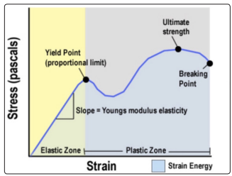
Figure 1: Stress-Strain-Young’s modulus, Elastic Zone vs. Plastic Zone
Nylon: 2.7 GPa
Concrete: 17-30 GPa
Glass fibers: 72 GPa
Copper: 117 GPa
Steel: 190-215 GPa
Diamond: 1220 GPa
Young’s modules in the above table are ranked from soft material (low E) to stiff material (higher E).”
Professor James Andrews taught the author linear elasticity at the University of Iowa and Professor Norman Jones taught him nonlinear plasticity at Massachusetts Institute of Technology. These two great academic mentors provided him the necessary foundation knowledge to understand these two important subjects in engineering.
In this particular study, he uses the analogy of relationship among stress, strain, and Young’s modulus to illustrate a similar relationship between body weight and predicted FPG via a newly defined coefficient of GH.f-modulus which is listed below:
= FPG / Weight
= stress / strain
Where FPG is the amount of predicted FPG (note: the predicted FPG can also be replaced by the measured FPG in order to conduct a sensitivity study of FPG behaviors).
Case A (the author) is a 73-year-old male with a 25-year history of T2D. From 7/1/2015 to 10/31/2020 (1,962 days), he has collected 2 data per day, weight and FPG. He utilized these data to conduct his linear elastic FPG behavior research.
In addition, on 5/5/2018, he started to use a continuous glucose
monitoring (CGM) sensor device to collect 96 glucose data each
day. Within this time period, he uses a sensor device to collect 28
FPG data per day from 00:00 to 07:00 at each 15-minutes time
interval. Based on his research, this averaged sensor FPG value
is within 1% of margin (i.e., 99% accuracy) from his measured
FPG at the wake-up moment using finger-piercing and test strip
method (Finger FPG).
The period of 7/1/2015 to 10/31/2020 is his “best-controlled”
diabetes period, where his average daily glucoses is maintained
at 116 mg/dL (<120 mg/dL). He named this as his “linear elastic
zone” of diabetes health.
Especially, due to his
It should also be noted that in 2010, his average glucose was
280 mg/dL and HbA1C was 10%, while taking three diabetes
medications. Please note that the strong chemical interventions
from various diabetes medications could seriously alter glucose
physical behaviors. He called the period prior to 2015 as his
“nonlinear plastic zone” of diabetes health.
The second set of data comes from his wife (Case B) with a 22-year history of T2D. She began to collect her glucose data via finger-piercing method (finger glucose) since 1/1/2014. On 1/1/2020, she began using the same brand of CGM sensor device to collect her sensor FOG data at the same rate of 28 FPG dataper day since 1/1/2020. She discontinued her diabetes medication in 2020.
Case C is 47-year-old male with a BMI over 40 (obesity) and a 4-year history of T2D (new and non-severe diabetes). He started to collect his glucose data using the same model of CGM sensor on 3/18/2020. He has never taken any diabetes medications. The following lists the different time spans of his four analysis:
(1) Case A:
From 1/1/2014 to 10/31/2020, every 6 months (semi-annually)
(2) Case B:
From 1/1/2020 to 10/31/2020, every month (monthly)
(3) Case C:
From 3/1/2020 to 10/31/2020, every month (monthly)
(4) Case A, Case B, and Case C:
From 3/1/2020 to 10/31/2020, every month (monthly)
He then calculates the value of GH.f-modules by dividing FPG by Weight for each time period. Using the averaged GH.f-modulus as a constant to plug it into the following equation to obtain the predicted FPG.
Finally, he compared the predicted FPG with the measured FPG to obtain prediction accuracies for each time period.
Figure 2 shows the raw data and the combined two charts, Weight versus FPG and the coefficient of GH.f-modulus, into one diagram for Case A (male patient with 14 semi-annual periods). His average weight is 173 lbs. and average FPG is 117 mg/dL. His average GH.f-modulus is a constant of 0.67 with a variance between 0.55 and 0.74. It should be noted that his significantly lower coefficient of 0.55 in the second half of 2020 is the direct result of his COVID-19 quarantined life. The compatible moving trend (i.e., high correlation) between weight and FPG over these periods is quite obvious. His average predicted FPG using the constant of 0.67 (i.e., a constant GH.f-modulus) is also 117 mg/dL, but with a variance range of FPG prediction error margin between -8% to +5%, excluding significantly positive contribution on his overall health conditions from a stabilized 2020 quarantined lifestyle.
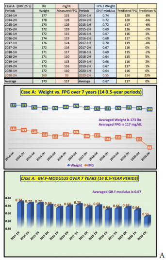
Figure 2: Case data & charts
Figure 3 depicts the raw data and the combined two charts, Weight versus FPG and the coefficient of GH.f-modulus, into one diagram for Case B (female patient with 10 monthly periods). Her average weight is 155 lbs. and average FPG is 104 mg/dL. Her average GH.f-modulus is a constant of 0.67 as well (same as Case A) with a variance between 0.63 and 0.70. It should be noted that her relatively more evenly distributed GH.f-modulus is due to the relatively smaller changes of her health conditions since 2010 instead of the 7-year-time period for Case A. The compatible moving trend (i.e., high correlation) between Weight and FPG over these 10 months is also quite evident. Her average predicted FPG using the constant of 0.67 (i.e., a constant GH.f-modulus) is also 104 mg/dL, but with a variance range of FPG prediction error margin between -5% to +6%.
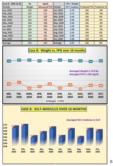
Figure 3: Case data & charts
Figure 4 illustrates the raw data and the combined two charts, Weight versus FPG and the coefficient of GH.f-modulus, into one diagram for Case C (younger male patient with 8 monthly periods). His average weight is 292 lbs. (extremely obese) and average FPG is 105 mg/dL (similar to Case B). His average GH.fmodulus is a constant of 0.36 due to his obesity, with a variance between 0.34 and 0.40. The compatible moving trend (i.e., high correlation) between Weight and FPG over these 8 months is also quite obvious. It should be highlighted that he has reduced his monthly average weight from 301 lbs. in January 2020 to 273 lbs. in October 2020. This significant weight reduction effort has assisted him with his average FPG reduction from 120 mg/dL in March 2020 to 95 mg/dL in October 2020. His average predicted FPG using the constant of 0.36 (i.e., a constant GH.f-modulus) is also 105 mg/dL, but with a variance range of FPG prediction error margin between -9% to +5%.
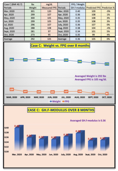
Figure 4: Case C data & charts
Figure 5 reflects the results of a special analysis by using a consistent time period (monthly data from 3/1/2020 to 10/31/2020) for Cases A, B, and C. The key objective of conducting this timeframe analysis is to compare their GH.f-modulus over the same 8-month-time frame.
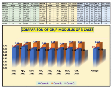
Figure 5: GH.f-modulus during the consistent 8-month time span of Cases A, B, and C
Listed below are the values of the GH.f-modulus for each patient over the 8-month period in 2020, which are listed in the order of Case A, Case B, Case C:
March 2020: (0.63, 0.64, 0.40)
April 2020: (0.66, 0.66, 0.36)
May 2020: (0.58, 0.69, 0.35)
June 2020: (0.58, 0.64, 0.35)
July 2020: (0.56, 0.68, 0.36)
August 2020: (0.58, 0.63, 0.38)
September 2020: (0.59, 0.68, 0.34)
October 2020: (0.56, 0.68, 0.35)
Although the coefficient changes from month to month, the magnitude of its changes are not significant. The results for Case C is the same as in Figure 4, but the results for Case B is smaller than in Figure 3 due to a shorter 8-month period used. The most significant difference is for Case A. The 14 semi-annual analysis has an average GH.f-modulus of 0.67, while his 8-month analysis has an average GH.f-modulus of 0.59. The 12% difference is a result from the different time spans chosen, which demonstrate the characteristics of organic blood material. There are more sources of influences than blood alone. In reality, weight and glucose are involved with many internal organs and hormones produced by the body.
Patients with varying chronic diseases would have different coefficient of GH.f-modulus. Both Case A and Case B are longterm T2D patients; however, their weights are still within the boundary of normal and slightly overweight with BMI around 25. Therefore, using 14 semi-annual periods for Case A and 10 months for Case B, their coefficients are the same at 0.67. However, due to Case A’s stringent lifestyle management to control his diabetes, his weight and glucoses, including FPG, have reduced significantly, especially in 2020 where his coefficient became 0.59 in comparison with Case B’s 0.66.
Case C is another story. His extreme-obese condition (BMI at
40.7) is much more serious than his diabetes conditions with
a 4 years of short history. In order to compensate for his heavy
weight, he must have a much lower value of the GH.f-modulus
(his coefficient of 0.36 is at 54% level of 0.67 for both Case A
and Case B) in order to match with his measured FPG level at
105 mg/dL (normal glucose level).
At first glance of this coefficient, it appears that it as a variable,
rather than a constant. However, by examining their values within
a reasonable time span, they do not vary that much. That is why it
is called a “pseudo-linear” relationship. Once we have collected
sufficient data for a particular time period, we can then easily figure
out the suitable coefficients for both FPG and PPG respectively,
i.e. GH.f-modulus and GH.p-modulus, to be used in glucose
predictions.
The article represents the author’s special interest in using mathphysical and engineering modeling methodologies to investigate
various biomedical problems. The methodology and approach
are a result of his specific academic background and various
professional experiences prior to the start of his medical research
work in 2010. Therefore, he has been trying to link his newly
acquired biomedical knowledge over the past decade with his
previously acquired knowledge of mathematics, physics, computer
science, and engineering for over 40 years.
The human body is the most complex system he has dealt with,
which includes aerospace, navy defense, nuclear power, computers,
and semiconductors. By applying his previous acquired knowledge
to his newly found interest of medicine, he can discover many
hidden facts or truths inside the biomedical systems. Many basic
concepts, theoretical frame of thoughts, and practical modeling
techniques from his fundamental disciplines in the past can be
applied to his medical research endeavor. After all, science is based
on theory from creation and proof via evidence, and as long as
we can discover hidden truths, it does not matter which method
we use and which option we take. This is the foundation of the
GH-Method: math-physics medicine.
The author has spent four decades as a practical engineer and
understands the importance of basic concepts, sophisticated
theories, and practical equations which serve as the necessary
background of all kinds of applications. Therefore, he spent his
time and energy to investigate glucose related subjects using
variety of methods he studied in the past, including this particular
interesting stress-strain approach. On the other hand, he also
realizes the importance and urgency on helping diabetes patients
to control their glucoses. That is why, over the past few years, he
has continuously simplified his findings about diabetes and try
to derive more useful formulas and simple tools for meeting the
general public’s interest on controlling chronic diseases and their
complications to reduce their pain and probability of death [5-9].