Author(s): <p>S. Azizu</p>
In this paper, analysis of some nonstationary iterative methods using the Vandermonde and Pascal linear system is reported. The nonstationary iterative methods selected were GMRES and QMR to assess their performance on the identified linear systems. The paper focused on the convergence relative residual and number of iteration for each type of chosen linear system. The Vandermonde matrix is mostly applied to interpolation of both quadratic and cubic polynomial function. The resulting polynomial has the form: p(x) = an xn + an-1xn-1 +...+ a1 x + a0. From the numerical experiments conducted using the matlab programming language, the GMRES is recommended when solving the identified linear systems
Pascal matrix mostly applied in real life situation is an infinite matrix containing the binomial coefficients as its main elements. This type of matrix is constructed by taking the matrix exponential of a special subdiagonal or superdiagonal matrix and this is achieved using three ways: as either an upper-triangular matrix, a lower-triangular matrix, or a symmetric matrix [1]. The Pascal matrix arises in many applications such as in binomial expansion, probability, combinatory, and linear algebra.
The Pascal matrix Pn [2] enjoys the following properties: (i) Pn is totally positive;
(ii) Pn is positive definite;
(iii) The eigenvalues of the matrix Pn are real and positive;
(v) det(Pn ) = 1;
The applications Vandermonde matrices are manifested in polynomial interpolation and Fourier transformations.
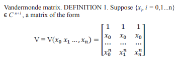
is called a Vandermonde matrix. A Vandermonde matrix is completely determined by its second row, and so depends on n + 1 parameters. All rows are powers of the second row from the power 0 to power n. Vandermonde matrices have a reputation of being ill-conditioned [3]. This reputation is well deserved for matrices whose nodes are all real, in which case the condition number is expected to grow exponentially with the order of the matrix and is also applied when we need to solve systems of differential equations [4]. This matrix often arise in engineering problems such as interpolation, extrapolation, super-resolution and recovering of missing samples [1]. The Vandermonde matrix in real life applications is an n x n matrix where the first row is the first point evaluated at each of the n monomials and the second row is the second point x2 evaluated at each of the n monomials.
Matrices play an important role in all branches of science, engineering, social science and management. Matrices are used for data classification by which many problems are solved using computers [2].
The relationship between inverse and confluent of Vandermonde matrices was presented [4]. Using symmetric functions and combinatorial identities to deduce the lower and upper triangular matrix of the inverse of the Vandermonde matrix has been studied [5]. These lower and upper triangular matrices are factorized completely into 1-banded [6]. In solving interpolation problem, new algorithm which is faster, accurate and which needs less storage for solving confluent Vandermonde systems has also been studied by and another algorithm is proposed to find its inverse in an explicit form where certain matrices built from Vandermonde matrices are of full rank [3,4,7].
The nonstationary iterative methods are standard iterative methods for solving sparse linear systems [8]. The conjugate gradient (CG) method is one of the most important acceleration methods in solving large and sparse symmetric. The CG algorithm, applied to the system Ax = b, starts with an initial guess of the solution x0 with an initial residual ro and with an initial search direction that is equal to the initial residual: p0 = r0 . The idea behind the conjugate gradient method is that the residual rk = b - A xk is orthogonal to the Krylov subspace generated by b, and therefore each residual is perpendicular to all the previous residuals. The residual is computed at each step. The solution at the next step is found using a search direction that is only a linear combination of the previous search directions, which for x1 is just a combination between the previous and the current residual. Then, the solution at step k, xk , is just the previous iterate plus a constant times the last search direction. Consider the problem of finding the vector x that minimizes the scalar function where the matrix A is symmetric and positive definite. Again f(x) is minimize when its gradient ∇f = Ax - b = 0. It implies that the minimization is equivalent to Ax = b. Gradient methods accomplish the minimization by iteration starting with an initial vector x0 . The approximate methods that provide solutions for systems of linear equations are called iterative methods. They start from an initial guess and improve the approximation until an absolute error is less than the pre-defined tolerance.
Iterative methods are suitable for very large systems of linear equations. These methods are very effective concerning computer storage and time requirements. One of the advantages of using iterative methods is that they require fewer multiplications for large systems. They are fast and simple to use when coefficient matrix is sparse. Advantageously they have fewer rounds off errors as compared to other direct methods
The Generalized Minimal Residual (GMRES) method computes a sequence of orthogonal vectors and combines these through least-squares method. This method combines with preconditioning as discussed earlier in order to speed up convergence. However, CG requires storing the whole sequence, so that a large amount of storage is needed. For this reason, restarted versions of this method are used. In restarted versions, computation and storage costs are limited by specifying a fixed number of vectors to be generated [9]. This method is useful for general nonsymmetric matrices. GMRES is the most popular Krylov subspace method applicable to any invertible matrix A.
A related algorithm, the Quasi-Minimal Residual method attempts to overcome this problem. The main idea behind this algorithm is to solve the reduced tridiagonal system in a least squares sense, similar to the approach followed in GMRES. Since the constructed basis for the Krylov subspace is bi-orthogonal, rather than orthogonal as in GMRES, the obtained solution is viewed as a quasi-minimal residual solution. Additionally, QMR uses look-ahead techniques to avoid breakdowns in the process [9].
In this paper, we present some numerical results to show the performance of nonstationary iterative methods using Vandermonde and Pascal matrix system. The convergence, condition number and relative residual for each system were computed and analyzed. We ran our algorithm using MATLAB software version 7.0.1 on Intel(R) Pentium (R) CPU P600 1.87GHz 1.87 and Installed Memory (RAM): 4.00GB. We considered the identified system of linear equations using the MATLAB command for the coefficient matrix A and RHS vector b where the exact solution is x = ones (n,1) for the discussion to test for the performance criteria. The 2-norm (Euclidean norm) of a vector is computed in MATLAB using function norm.
Table 1: Pascal System n= 10
| NONSTATIONARY ITERATIVE METHODS | |||
|---|---|---|---|
| Methods | Flag | No. of Iteration | Relative Residual |
| GMRES | 0 | 6 | 2.8e-008 |
| QMR | 0 | 7 | 3e-008 |
Table 2: Pascal System n= 20
| NONSTATIONARY ITERATIVE METHODS | |||
|---|---|---|---|
| Methods | Flag | No. of Iteration | Relative Residual |
| GMRES | 0 | 4 | 5.7e-007 |
| QMR | 0 | 5 | 5.7e-007 |
Table 3: Pascal System n= 30
| NONSTATIONARY ITERATIVE METHODS | |||
|---|---|---|---|
| Methods | Flag | No. of Iteration | Relative Residual |
| GMRES | 0 | 4 | 9.6e-008 |
| QMR | 0 | 5 | 9.6e-008 |
Table 4: Pascal System n= 100
| NONSTATIONARY ITERATIVE METHODS | |||
|---|---|---|---|
| Methods | Flag | No. of Iteration | Relative Residual |
| GMRES | 0 | 3 | 6.9e-008 |
| QMR | 0 | 3 | 6.9e-008 |
Table 5: Pascal System n= 200
| NONSTATIONARY ITERATIVE METHODS | |||
|---|---|---|---|
| Methods | Flag | No. of Iteration | Relative Residual |
| GMRES | 0 | 3 | 8.4e-009 |
| QMR | 0 | 3 | 1.8e-008 |
Table 6: Vandermonde System n=10
| NONSTATIONARY ITERATIVE METHODS | |||
|---|---|---|---|
| Methods | Flag | No. of Iteration | Relative Residual |
| GMRES | 0 | 5 | 1.9e-007 |
| QMR | 0 | 6 | 4.4e-008 |
Table 7: Vandermonde System n=20
| NONSTATIONARY ITERATIVE METHODS | |||
|---|---|---|---|
| Methods | Flag | No. of Iteration | Relative Residual |
| GMRES | 0 | 4 | 2.2e-007 |
| QMR | 0 | 11 | 2.6e-008 |
Table 8: Vandermonde System n= 30
| NONSTATIONARY ITERATIVE METHODS | |||
|---|---|---|---|
| Methods | Flag | No. of Iteration | Relative Residual |
| GMRES | 0 | 2 | 5.7e-007 |
| QMR | 0 | 12 | 8.3e-009 |
Table 9: Vandermonde System n=100
| NONSTATIONARY ITERATIVE METHODS | |||
|---|---|---|---|
| Methods | Flag | No. of Iteration | Relative Residual |
| GMRES | 0 | 2 | 3.9e-009 |
| QMR | 1 | 20 | 0.043 |
Table 10 : Vandermonde System n=200
| NONSTATIONARY ITERATIVE METHODS | |||
|---|---|---|---|
| Methods | Flag | No. of Iteration | Relative Residual |
| GMRES | 1 | 0 | NaN |
| QMR | 1 | 2 | NaN |
Nonstationary iterative methods (GMRES and QMR) were presented using Vandermonde and Pascal linear systems. From the numerical experiments conducted using the matlab programming language, the GMRES is recommended when solving the identified linear systems. The two methods did not converge when the number of sizes for the named system is 200. Only GMRES converges when the matrix size is 100. The future work is to consider incorporating the identified nonstationary iterative methods with some acceleration schemes to assess the convergence of higher matrix for both Vandermonde and Pascal linear system.